Excel 2016: How to Format Cells and Worksheets

Creativity and uniformity are few of the least aspects most people consider in using Excel. More often, we tend to disregard the styles we use, for instance fonts, no matter how different they are from each other. We ignore the format, most especially when we are working with lots of information in a worksheet. However, formatting your worksheets is not a difficult task at all. Doing so will make your file look more organized and professional. Uniformity will even encourage you to work on your file with enthusiasm and excitement.
The Home Ribbon to customize and format cells and worksheets
Excel 2016 consists of several ribbons that make you do complicated tasks in just few clicks. One of them is the Home Ribbon. This portion contains mostly of formatting and editing tools.
The Main Groups in Excel 2016 Home Ribbon
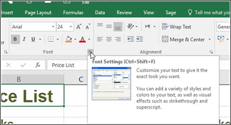
1. Font Group
This group contains the main features for changing the appearance of your content, as shown below.
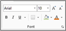
Using the font group, you will be able to change the font style and size of the contents of your cell. Just follow the steps below.
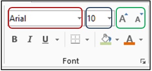
- Go to Home Ribbon and look for the Font Group.
- Select the cell/s you want to format.
- Click on the drop down arrow next to the font style (red) or font size (blue) box.
- Select the font style or font size you require.
Note: Changing the font size is also possible just by clicking the “grow and shrink font” button, enclosed in green.
You can also make your contents be boldfaced, italicized or underlined in just a click.
- Select the cell/s you want to format.
- Click on the icon you require.
![]()
For more detailed changes, you can explore the font settings by following the steps below.
- Select the cell/s you want to format.
- Click on the Dialog box launcher arrow.
- Make the changes you require.
- Click OK.
2. Alignment Group
This group indicates where your text/numbers will line up in a cell.
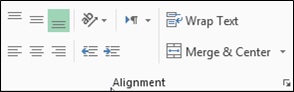
Setting the Alignment
- Click on the cell/s you want to format.
- Click on the icon you require.

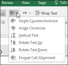
Text/ Number Orientation
You can also change the direction of text in a cell/s by simply selecting the cell/s to change and then choose the orientation you need.
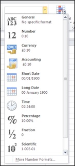
3. Number Group
Number group allows formatting of your figures. It has shortcuts for a particular number format, like adding currency – which could be GBP, Dollars or the Euro symbol, formatting a number as a percentage, adding a thousand separator or increasing/ decreasing decimals.
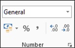
To apply number format
- Select the cell/s you want to format.
- Click the drop down arrow.
- Choose the format you need.
To remove number format
- Select the cell/s you want to clear the format.
- Click the drop down arrow.
- Choose the first option – General (No Specific Format).
Other Important Features…
4. Wrap Text
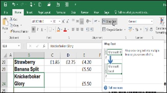
This feature helps you add more text in the cell by increasing its height but keeping its width. It is useful if you have text that is too wide for the cell.
- Select the cell you want to wrap.
- Go to the Alignment Group on the Home Tab.
- Click on Wrap Text button.
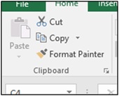
5. Format Painter
This feature allows you to copy the formatting from one part of your workbook to another.
Using Format Painter Once
- Select the cell that contains the formatting you want to copy.
- In the Clipboard group of the Home ribbon, click on the Format Painter button.
- Click on the cell (or click and drag on the cells) you want to apply the formatting.
Using Format Painter to copy to more than one cell
- Select the cell that contains the formatting you want to copy.
- In the Clipboard group of the Home ribbon, double click the Format Painter button.
- Click and drag over the text you want to use the format with.
- Click on the Format Painter button once again to switch it off.
Formatting your calls and worksheets is not hard at all. The Home Ribbon allows you to do it in just a few clicks. You will only have to select the cell/s you want to format, then click on the command button you need – it’s just that simple!
We have even more useful articles:
Excel 2016: 3 Simple Steps to Hide and Unhide Portions
“Essential Facts About Worksheets and Workbooks and How to Utilize Them”