Excel 2016: How to Split Cells in Excel for a Better View

How to make your work easier when splitting large worksheets

Working on a huge workbook that has significant information all throughout its part is very tedious and time-consuming; especially when you are constantly scrolling up, down, left and right just to see and work at different parts.

Well, worry no more! By using the different views of Excel 2016, you will be able to save lots of time and effort in manipulating your workbooks and worksheets.
Imagine you have two copies of a worksheet and you are able to control both of them independently or two different worksheets of a single workbook both seen on your screen. Then, whatever you do on the first copy will be automatically applied to the other one. Isn’t that great? How is that possible? Simply because you’re really working on ONE worksheet which only appears double on your screen at the same time. Now, that’s incredibly amazing!

Splitting the Window

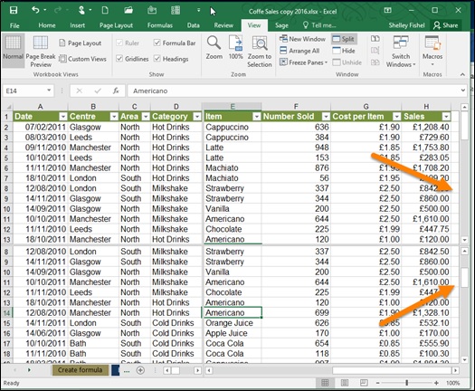
In using this option, the worksheet will split above and to the left of where your cursor is.

1. Click on the worksheet where you want to split the worksheet.
2. Click on the View tab.
3. Click the Split button.
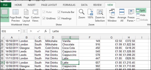
4. You can now scroll in the top or the bottom half, just like below:

How to remove the split?

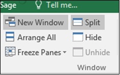
1. Click on the View tab.
2. Click on Split. (as shown below)

Opening Two Copies of the Same Workbook

When working with Excel, there are times that you need to view two worksheets of the same workbook at the same time. For instance, you have a summary worksheet and you need to see the effect of making a change on one of the spreadsheets that feed into it. To make things easier, you can open a second copy of the workbook in a new window and then arrange the windows side by side so that you can see both of them. Whenever you make a change on the first worksheet, you will be able to see the effect on the other one. Indeed, a very powerful feature! How to do it? Follow the steps below:

1. Go to the View Ribbon.
2. Click on New Window.
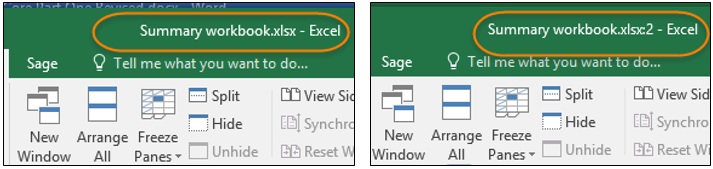
3. A new window will appear.

4. Go to the View Ribbon
5. Click on Arrange All and a dialog box will appear.

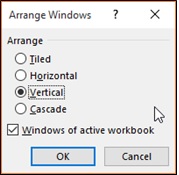
4. Select the way you wish to see the worksheets arranged.
5. Tick Windows of active workbook.
6. Click OK.

In this example, vertical is selected. Now, there are two copies that are arranged side by side.

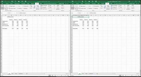
With this view, you will be able to work quickly and easily since both of the worksheets that you need are on sight.

Try it and enjoy working!

We have even more useful articles:

• Basic Excel Functions: SUM, AVERAGE, MAX, MIN and COUNT
• How to Copy Formulas in Excel
• Get Faster Using the Flash Fill Feature
• Save Time Using Autofill
• 3 Simple Steps to Hide and Unhide Portions
• How to Format Cells and Worksheets
• Essential Facts About Worksheets and Workbooks and How to Utilize Them
• Customize The ‘Quick Access Toolbar
• How to Use Excel’s Basic Functions