Remarkable features of the quick access toolbar in Excel 2013


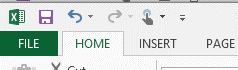
Each of the Office packages including Word, Excel, PowerPoint and Outlook has an amazing feature called Quick Access Toolbar. This feature holds the frequently used shortcuts in each program. It can be found on the uppermost left corner of the screen, just above the File menu. In Excel, the Quick Access Toolbar looks like the image below.
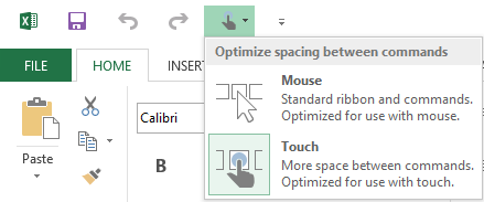
Originally, the toolbar is composed of these icons: Save, Undo, Redo and Touch. The purpose of the Touch option is to change the spacing of icons in the Ribbon giving more space between icons for use with a touch device. However, this can also be changed into Mouse icon, which has a standard spacing for devices with mouse, as seen below.
Customizing the Quick Access Toolbar
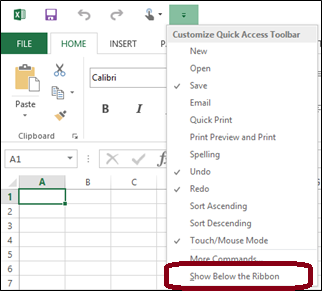
The Quick Access Toolbar can be customized based on your own preference. You can add or remove icons depending on your own need. You can also move it below the Ribbon so that more space will be available if you will add more icons in it. To do so, just click the drop down arrow and click the option “Show Below the Ribbon” and your toolbar will instantly move.
[bookboon-book id=”9790ac2b-f06b-4a05-a20e-a34800d72aee” title=”Check out the Excel 2013 guide” button=”Read eBook”]
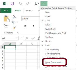
If you want to add icons in the Quick Access toolbar, you just have to click the drop down arrow and choose between the standard icons there. Option includes New, Open, Email, Quick Print, etc. You can also choose the “More Commands…” option for more choices. Same procedure should be done on removing icons. In the standard choices, you will just have to tick or uncheck the icon you want to remove or choose and click Remove in the “More Commands…” option.
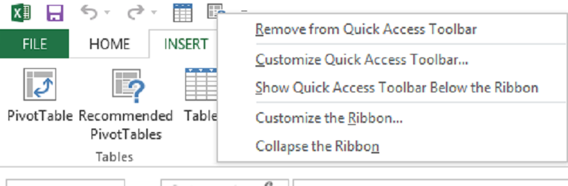
You can also add icons through right click. If you happen to notice that an icon is frequently used, you just have to click on the Right Mouse button and choose the option to add it on your Quick Access Toolbar, just like below.
You can also remove an icon in the Quick Access toolbar using this procedure. Just click the Right Mouse button and click “Remove from Quick Access Toolbar” option.
Exploring Hundreds of Commands in Excel
Different people use Excel differently. Therefore, it is very natural that we have different options and choices when it comes to adding icons in the Quick Access Toolbar. There are hundreds of icons available in Excel, same as with other Office programs. You can explore them all by choosing the “More Commands…” option in the drop down arrow.
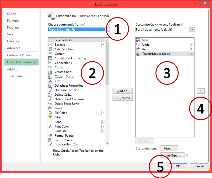
- Icons have different categories. You can choose between these categories and have a look through the available icons in each.
- This column shows the available icons in your chosen category displayed – double click an icon or click the “Add >>” button to place it in your Quick Access toolbar.
- This shows the icons currently on the Quick Access Toolbar. You can remove an icon by clicking the “Remove >>” button.
- These spinners will let you move and order the icons up and down.
- When everything is done, just click OK and your Quick Access toolbar is ready.
Shortcut Keys Using the Alt Key and the Quick Access Toolbar
Excel 2013, and other features of the Office 2013, comes with a built-in shortcuts that can be accessed using the Alt key. Once you press the Alt key, numbers will appear in the Quick Access toolbar (while letters in each ribbon), just like below.
Once you pressed the Alt Key plus the number, it will do the corresponding task. Let’s say Alt + 1, the document will be saved, Alt + 2 will undo, etc. Using the Alt key and the Quick Access toolbar will let you save substantial amount of time in using Excel 2013.
We hope you enjoyed this blog post and it helps you with your work in the future. Please also have a look at our other Excel blogs “Best Excel 2013 tricks: Naming a Cell” and “How to quickly create a chart in Excel“. Don’t forget to check out our other Microsoft Office blogs.
Let us know if you like the blog and post your best tips and tricks below. Don’t forget to share this article with your colleagues and friends!
[bookboon-recommendations id=”9790ac2b-f06b-4a05-a20e-a34800d72aee” title=”You might also find these books interesting…”]