How to use the IF Function in Excel
One of the reasons Excel is such a practical tool are its formulas. In this article we will show you how to apply conditional logic in formula. Find out how to use the IF Function, nested IF Function, COUNTIF Function and SUMIF Function. Please read on…
IF Function (IF Statement)
An If function asks Excel to consider if something is true or false. If it is true it will return one answer, if it is false it will return a different answer.
For example: Can my company afford to buy 10 new computers? There are 2 possible outcomes – if it is within the budget then the answer is “yes”, if it is outside of the budget then the answer is “no”.
The structure of an IF Function
=IF(B6<=$B$3,“yes”,“no”)
The structure of an IF statement always contains the same five elements.
- Starts with =IF(
- The Logical Test followed by a comma
- What to do if the logical test is True followed by a comma
- What to do if the logical test is False
- Close brackets
To make this IF function easier to understand the logical test is in one colour, the true part is in another colour and the false part is in a third colour.
Operators you can use in a Logical Test
| Operator | Explanation |
| = | Equal to |
| <> | Not equal to |
| > | Greater than |
| < | Less than |
| >= | Greater than or equal to |
| <= | Less than or equal to |
Typing in an IF Function
Figure 1- structure of an IF statement
- Click in the cell where you want the answer
- Type in the =IF(
- Type in your logical test
- Type a comma
- Type in what Excel must do if this is true
- Type a comma
- Type in what Excel must do if this is false
- Close the brackets
- Press Enter
If Excel is to display text for the true or false result then you must enclose the text in inverted commas.
You can also put a formula in the IF statement for the True or False result.
For example:
I want to know how much bonus each member of staff will receive:
=IF(B2>$H$1,C2*$h$2,0)
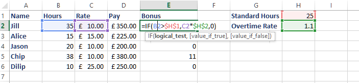
Figure 2- working out the bonus amount
Nested IF Function
A nested IF Function is an IF function nested inside another IF function.
The basic IF function only allows for two possible answers: either the logical test is met or it is not. When we want more than these two basic answers then we need to nest the formula, i.e. put one =IF inside another.
You can nest up to sixty four IF functions inside one another, but if you were going to go so far, you would be more likely to use a HLOOKUP or VLOOKUP.
The structure of a nested IF Function
=IF(B5>=$G$2,”OAP”,If(B5<=$G$3,”Child”,”Adult”))
A nested IF Function is just a lot of single IF functions strung together. The structure of nested IFs is always as follows:
- Startwith =IF(
- First logical test followed by a comma
- What to do if the first logical test is true
- If the first logical test is false then Excel has to move onto the next logical test which will always start with IF(
- Second logical test followed by comma
- If the second logical test is also false Excel moves onto the next logical test and this process repeats until you come to the last logical test
- At the end of the nested IF there will be your last logical test
- What to do if the last logical test is true
- What to do if the last logical test is false
You must type in a closing bracket at the end of the nested IF for each logical test you have entered.
COUNTIF Function
The COUNTIF function combines the COUNT function and the IF function. Use it when you want to count any cells that match a certain condition.
Figure 3-count how many people have overtime
In the example, we want Excel to count how many people have worked enough hours to qualify for overtime. So we set up a COUNTIF Function to count how many times the word “Overtime” occurs in the Overtime column.
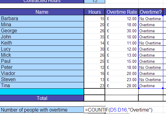
Figure 4- result returned
The structure of a COUNTIF Function
=COUNTIF(C6:C9,”yes”)
This says, look in the cells C6 to C9, and if you find the work yes in them count how many times.
The structure of a COUNTIF always contains the same four elements.
- Starts with =COUNTIF(
- The range of cells that Excel is to look at
- The criteria which Excel will use to count
- Close brackets
To make this COUNTIF function easier to understand in this example, the range is in purple text and the criteria is orange text.
Typing in a COUNTIF Function
![]()
Figure 5- type the Countif function directly into the cell
- Click in the cell where you want the answer
- Type =COUNTIF(
- Highlight the range of cells you are counting from
- Type in your criteria
- Press Enter
SUMIF Function
This function will add the value of cells that meet a certain criteria.
For example, suppose we want to calculate the total salary cost of all females:
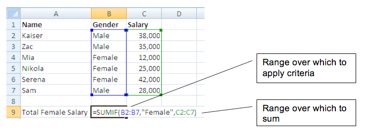
Figure 6- Sumif adds up all the rows that meet your criteria
If the range B2 to B7 says Female then add up all of the salaries that correspond.
The answer for the Total Female Salaries = £79,000.
The structure of a SUMIF Function
The syntax for the SUMIF function is as follows:
=SUMIF(Range,Criteria,Sum Range)
Range: The range of cells that Excel is to look at
Criteria: The criteria that the cells must meet in order to be added
Sum Range: The cells to Sum
We hope you found this article helpful and learned something new. Don’t forget to share it with your friends or colleagues if you think they could benefit from this article. You might also want to check out other Excel blogs such as “How to assign shortcuts in Excel 2013”, “Remarkable features of the quick access toolbar in Excel 2013” or “How to make Excel files compatible with older MS Office versions” and “How to add value to workbooks in Excel“.