How to use Quick analysis in Excel

Quick analysis is a new feature in Excel 2013. Quick analysis looks at the data you have selected and offers you various options to analyze and summarize the data. Once you get used to using it, you will wonder what you did before! Check out our easy steps to Quick analysis below…
There are five main types of analysis and within each type you will be offered more options.
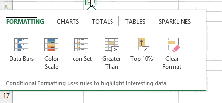
Figure 234-various quick analysis options
The main types of analysis are:
Formatting – here you can find various conditional formats – Excel will guess which are best suited to the data selected
Charts – A selection of charts will be suggested
Totals – Various calculations
Tables – A selection of tables will be found here
Spark lines – Excel will offer you spark lines to be added to adjacent cells
Quick analysis Formatting
Formatting
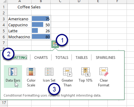
Figure 235- format data quickly
- Click the Quick Analysis Smart Tag
- Click on Formatting
- Choose from the formats offered – Excel will preview the chosen format on the selected data so you can flip between them before making a decision
Quick analysis totals
With the totals quick analysis you are offered a selection of functions that can be performed on the data. Choose whether to add them underneath the data or in a column to the right
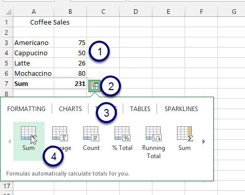
Figure 236- quick summaries
- Select the data
- Click the Quick Analysis Smart Tag
- Click on Totals
- Choose the type of total you want to add – Here I selected a Sum note that Excel added a total row to the data with the word Sum and also added the formula to the data
Quick analysis Charts

Figure 237- charts are offered too
- Select the data
- Click on the Quick Analysis Smart Tag
- Click on Charts
- Hover over the different charts to see a preview of how they will look – to select one click on it
- The chart is then placed on the spreadsheet – see below
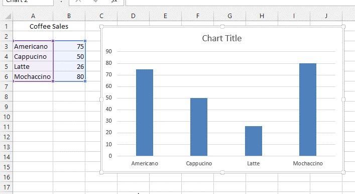
Figure 238- chart
Quick analysis Tables
Instead of selecting the data and choosing Format as Table from the Home Ribbon you can use quick analysis to get a standard table or a quick pivot table

Figure 239- quick tables
- Select the data
- Click the Quick Analysis Smart Tag
- Click on Tables
- Click Table and a preview will be placed over the data – click to insert
If you choose Blank Pivot Table, you will find a new blank pivot table inserted on a new worksheet ready for you to build
We hope you found this article helpful and learned something new. Don’t forget to share it with your friends or colleagues if you think they could benefit from this article. You might also want to check out other Excel blogs such as “How to manipulate illustrations in Excel”, “Remarkable features of the quick access toolbar in Excel 2013” or “How to make Excel files compatible with older MS Office versions” and “How to use the IF Function in Excel“.