How to quickly create a chart in Excel
Does this scenario sound familiar to you? You have just finished your report and are under time pressure. All you need now is a nice chart to visualise your results. Surely you have created charts in Excel in the past but you cannot remember the exact steps. Don’t panic!
We have put together a few easy steps for you to create a quick chart in Excel. It doesn’t require much time and can be used for all sorts of different data. Graph, line or pie chart, the choice is yours!
Follow these steps to create your Excel chart.
Quick Analysis Charts
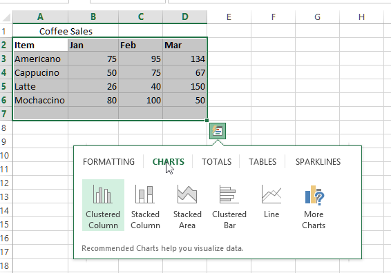
- At first you need to select the data.
- Then click on the small Quick Analysis button.
- Choose Charts and then hover over the different recommended charts to see what they look like.
- Find the one that does the job and click on it.
Recommended Charts
Excel is a practical tool and used in different jobs across many sectors. Some might even suggest it is the key to a good-paying job.
That’s why we have some more tips on charts here, please read on.
When creating a chart, it is sometimes a challenge to decide which chart type to use. In Excel 2013, you can now get a recommendation and see samples of the charts that Excel thinks fit your data. It is quite useful to see what it looks like before deciding if it is the right one for you.
Let Excel recommend a chart
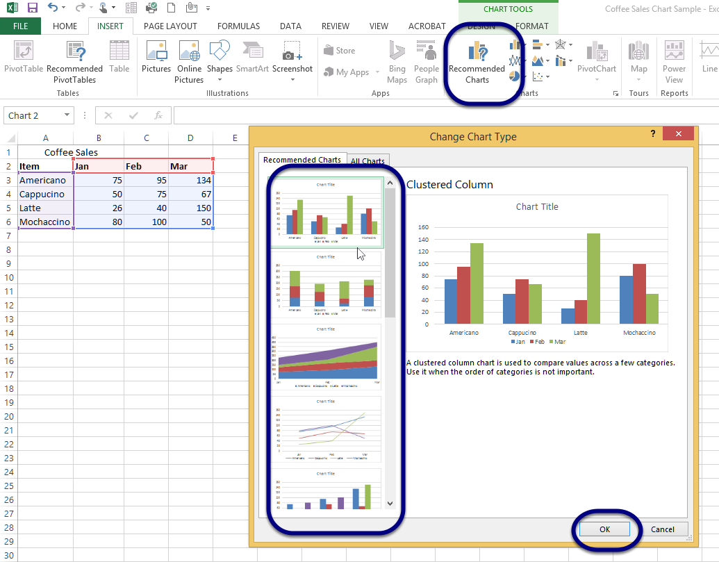
- Select the data for the chart
- Click on the Insert Ribbon
- Click on Recommended Charts
- Choose one of the charts that Excel suggests
- Click OK
The chart appears – magic!
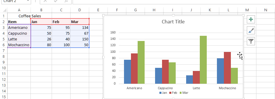
The chart type selected now appears on the spreadsheet next to the data, ready for a Chart Title or to be reformatted to match your style.
This wasn’t too difficult was it? If you would like to further customise your chart and change colours or font, just click on the symbols to the right. Clicking on the paintbrush button will open a window where you can make the desired changes. Have a look at other articles in this series such as “Best Excel 2013 tricks: Naming a Cell” or “Best Word 2013 tricks: Understanding the review tab“.