Best Excel 2013 tricks: Naming a Cell

Most of us are required to do calculations, reports or draw up a simple graph at some point in our careers. When that point comes it is handy to know a few tricks for using Excel to make your work easier.

Knowing how to name a cell or a range of cells is one of the things that will make your life easier when working in Excel and it is especially practical when using formulas in Excel.

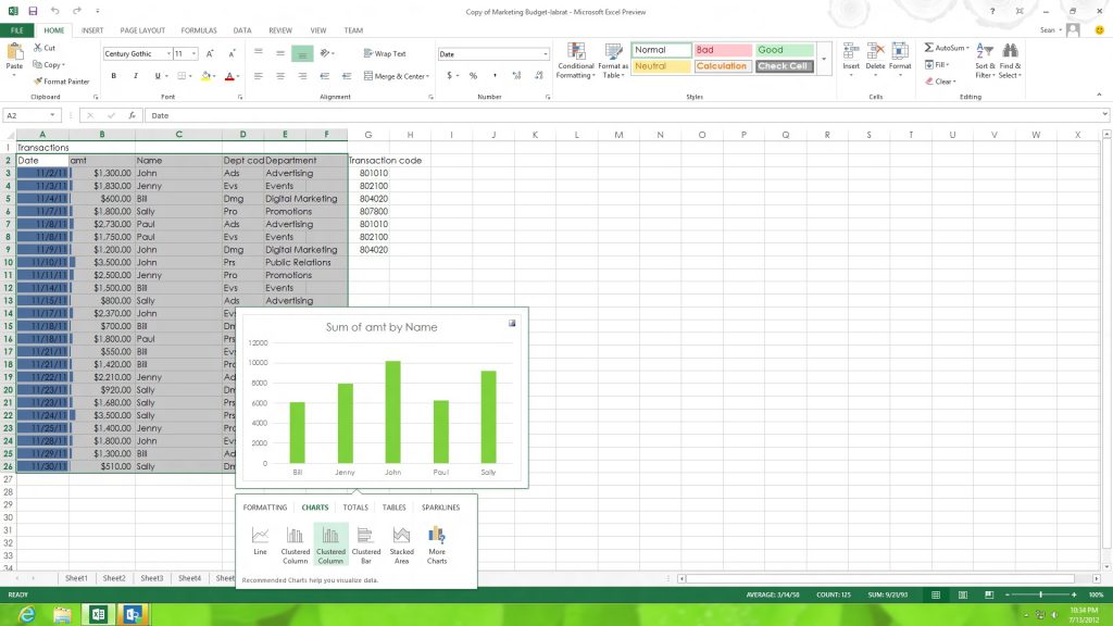
Naming a cell or range of cells can help in different ways. When a cell is named it behaves as an Absolute Cell Reference, by giving the cell a name such as VAT or Price, Excel knows to refer to that particular cell when you use it in a formula. Learn more Excel tricks, have a look at “How to create a chart quickly in Excel 2013“.

Name a range of cells and you can navigate around easily. When used in a formula Excel will pick up the right cell in the formula.

Named Ranges are also handy for summarizing data quickly or finding a piece of data at the intersection between two ranges. Read on to learn how this works.

But at first you have to open your Excel worksheet:

How to name a single cell

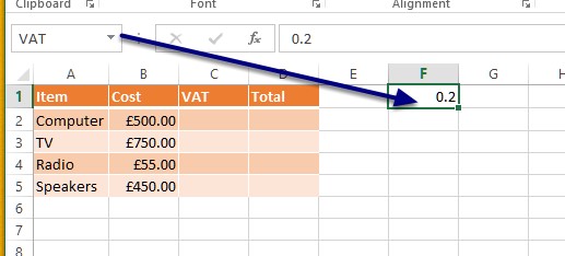
1. Click on the cell you want to name (in our example F1)

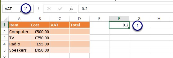
2. Click into the Name Box (to the left of the Formula Bar)

3. Over type the cell reference with the Name for the cell (In our example VAT)

4. Press Enter to confirm the name

Now I have a cell called VAT which can be seen from the drop down arrow in the Name Box

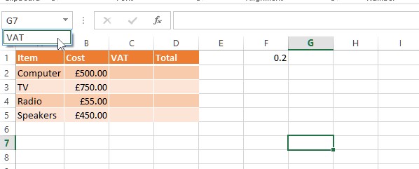
Here you can see that my cursor is in Cell G7 and in the drop down arrow is the name VAT.

To move the cursor to the cell called VAT I can select it from the drop down list.

Here you can see that I have now jumped to the cell called VAT and this is where the cursor is now positioned.

Now you have given your cell a name. Well done!

In this next section I will show you how you can use this named cell or range of cells in a formula.

Using a named cell in a formula

The advantages of a named cell in a formula are:

• it makes it more readable
• you can use it as an Absolute Cell Reference

To use the named cell in a formula you just have to follow these simple steps:

Create the formula as you normally would.

1. Click into the cell where the result will display
2. Type an = sign
3. Click on the first cell to include
4. Type the mathematical Operator ( in our example an Asterix for multiply)
5. Click on the cell with the multiplier in (F1 which is called VAT ) Notice that Excel calls the cell by its name not the cell reference
6. Press Enter

Auto fill the formula

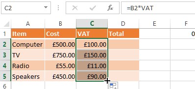
Use the Auto fill Handle (the little black plus sign in the bottom right hand corner of the cell to copy the formula down all the other rows.

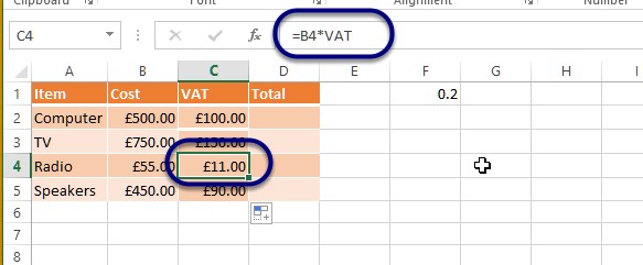
Notice that each of the rows has adjusted the first part so B2 then B3 then B4 etc however all of the formula reference the cell called VAT.

Now you know how to name a cell and use it in a formula. I wish you good luck with your next Excel report!
To find more helpful Excel 2013 tips, check out Shelley Fishel’s eBook “Excel 2013: Core Advanced” at bookboon.com. Don’t forget to check out other blogs in this series, such as “Understanding the review tab” and “How to insert tabs in Word 2013“.

[bookboon-book id=”f4cecc3d-5df2-4667-9daf-a34800dc266a” title=”More Excel 2013 tips in this eBook” button=”Read eBook”]