MS Excel 2016: Get Faster Using the Flash Fill Feature

How to use the Flash Fill feature in Microsoft Excel
Previously, when you have a data in columns and you want to combine them in a single cell, you need to create a formula. Formula must also be created when you want to extract data in a cell or format cells based on your reference. Well, the agony of creating formula for these tasks has now come to an end.
With Excel 2016, you can now make these complicated things simple through the feature known as Flash Fill. This feature was actually first introduced in Excel 2013 and I bet everybody enjoyed using it!
Trick Number 1: Flash Fill to Join Two Columns
In this example, we wanted to join the contents of the cells of “First Name” and “Last Name” in the cell of “Full Name”.
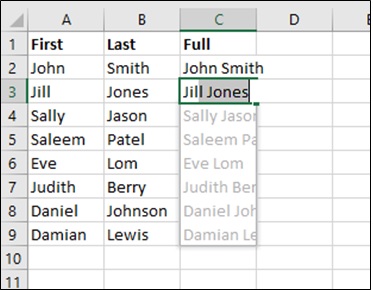
Seeing the picture above, you might be shocked with how Excel 2016 has made your agony of using formula in joining these contents fade away. You might not believe it at first but, yes, it is possible! How? Follow the steps below.
- Type the result you want in the first cell.
- Type the result you want in the second cell so Flash Fill gets to really work out what you are doing.
- You will see the grey suggestions.
- If you like what you see, simply press the Enter key and that’s it!
Trick Number 2: Flash Fill to Extract Data
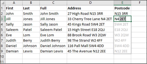
In this example, we wanted to extract the postcode in the Address and place it in a separate column.
You may do so by following these steps:
- Type a heading and format it in the first cell (E1 in this example).
- Type the first Postcode in the list.
- Start to type the second Postcode.
- Excel now finds the pattern in what you are doing and Flash Fills the rest of the column!
- Press Enter to accept.
Trick Number 3: Flash Fill to Format Telephone Numbers
In this example, we are given list of telephone numbers and we wanted to format it to have hyphens in between each block of numbers.

You may do so by following these steps:
- Format the cells as Text – this makes sure that any leading 0 stays put and does not get dropped.
- Format the cells in the next column as text too.
- Type in the first telephone number in the format you want to use.
- Start to type the second one.
- The Flash Fill suggestions will appear.
- Click Enter to accept.
These are just a few of the many tricks that you can do using the Flash Fill. Just like Autofill option, you can save lots of time and effort in doing your usual job with this useful feature of Excel 2016.
Now, you can say goodbye to complicated formulas and redundant tasks!
We have even more useful articles:
“3 Simple Steps to Hide and Unhide Portions”
“How to Format Cells and Worksheets”
“Essential Facts About Worksheets and Workbooks and How to Utilize Them”