Excel 2010 Advanced: What you ought to know about lookup functions in Excel

Knowing your way around Excel will definitely improve your work-rate and overall efficiency. But how skilled are you really in Excel? Below you can find an extract of the eBook “Excel 2010 Advanced” which you can download for free. Take a look and see whether you find the provided information useful. Read, download and bring your Excel skills up to a new level!

Insights into lookup functions

Excel can produce varying results in a cell, depending on conditions set by you. For example, if numbers are above or below certain limits, different calculations will be performed and text messages displayed. The usual method for constructing this sort of analysis is using the IF function.

However, this can become large and unwieldy when you want multiple conditions and many possible outcomes. To begin with, Excel can only nest seven IF clauses in a main IF statement, whereas you may want more than eight logical tests or “scenarios.” To achieve this, Excel provides some LOOKUP functions. These functions allow you to create formulae which examine large amounts of data and find information which matches or approximates to certain conditions. They are simpler to construct than nested IF’s and can produce many more varied results. Below you can take a closer look at three of the most common Lookup functions: the Vector Lookup, Hlookup and Vlookup.  

Before you actually start to use the various LOOKUP functions, it is worth learning the terms that you will come across, what they mean and the syntax of the function arguments.

Vector Lookup

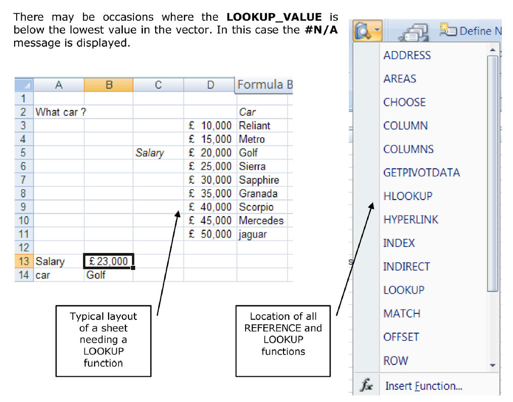
A vector is a series of data that only occupies one row or column. LOOKUP will look through this row or column to find a specific value. When the value is found, a corresponding “result” in the adjacent row or column is returned. For example, column D of a spreadsheet may contain figures, and the adjacent column E contains corresponding text. LOOKUP will search for the requested figure in column D and return the corresponding text from column E.

The syntax for LOOKUP is as follows;

=LOOKUP( lookup_value , lookup_vector , result_vector )

The LOOKUP_VALUE represents the number or text entry to look for; the LOOKUP_VECTOR is the area in which to search for the LOOKUP_VALUE; the RESULT_VECTOR is the adjacent row or column where the corresponding value or text is to be found.

It is essential that data in the lookup vector is placed in ascending order, i.e. numbers from lowest to highest, text from A to Z. If this is not done, the LOOKUP function may return the wrong result.

In the diagram, column D contains varying salaries, against which there is a company car in column E which corresponds to each salary. For example, a £20,030 salary gets a GOLF, a £35,000 salary gets a SCORPIO. A LOOKUP formula can be used to return whatever car is appropriate to a salary figure that is entered. In this case, the LOOKUP_VALUe is the cell where the salary is entered (B13), the LOOKUP_VECTOR is the salary column (D3:D11), and the RESULT_VECTOR is the car column (E3:E11). Hence the formula;

=LOOKUP(B13,D3:D11,E3:E11)

Typing £40,000 in cell B13 will set the LOOKUP_VALUE. LOOKUP will search through the LOOKUP_VECTOR to find the matching salary, and return the appropriate car from the RESULT_VECTOR, which in this case is MERCEDES.

Alternatively, the formula could be simplified and cell references avoided by using Formula, Define Name to give appropriate range names. Call B13Salary, D3:D11Salaries and E3:E11Cars. The LOOKUP formula could then be simplified to;

=LOOKUP(Salary,Salaries,Cars)

One of the advantages of the LOOKUP function is that if the exact LOOKUP_VALUE is not found, it will approximate to the nearest figure below the requested value. For instance, if a user enters a Salary of 23000, there is no figure in the Salaries range which matches this. However, the nearest salary below 23000 is 20030, so the corresponding car is returned, which is a Golf. This technique is very useful when the LOOKUP_VECTOR indicates grades or “bands.” In this case, anyone in the salary “band” between 20030 and 25000 gets a Golf. Only when their salary meets or exceeds 25000 do they get a SIERRA.

To insert a lookup function:

Mouse

1. Click the drop down arrow next to the LOOKUP AND REFENCe button in the FUNCTION LIBARY groupon theFORMULAS Ribbon;

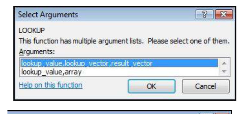
2. A dialog box appears displaying the two versions of LOOKUP. There are two syntax forms; the first is the “VECTOR” and the second the “ARRAY”

3. Choose vector and click ok

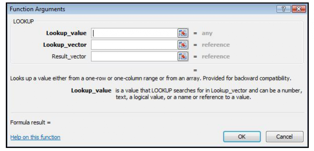
4. Enter the values as described previously and click OK

The first of these forms, the “vector” LOOKUP is by far the most useful, and it is recommended that you only use this form.

Hlookup

The horizontal LOOKUP function (HLOOKUP) can be used not just on a “VECTOR” (single column or row of data), but on an “array” (multiple rows and columns). HLOOKUP searches for a specified value horizontally along the top row of an array. When the value is found, HLOOKUP searches down to a specified row and enters the value of the cell. This is useful when data is arranged in a large tabular format, and it would be difficult for you to read across columns and then down to the appropriate cell. HLOOKUP will do this automatically.

The syntax for HLOOKUP is;

=HLOOKUP( lookup_value , table_array , row_index_number)

The LOOKUP_VALUE is, as before, a number, text string or cell reference which is the value to be found along the top row of the data; the TABLE_ARRAY is the cell references (or range name) of the entire table of data; the ROW_INDEX_NUMBER represents the row from which the result is required. This must be a number, e.g. 4 instructs HLOOKUP to extract a value from row 4 of the TABLE_ARRAY.

It is important to remember that data in the array must be in ascending order. With a simple LOOKUP function, only one column or row of data, referred to as a vector, is required. HLOOKUP uses an array (i.e. more than one column or row of data). Therefore, as HLOOKUP searches horizontally (i.e. across the array), data in the first row must be in ascending order, i.e. numbers from lowest to highest, text from A to Z. As with LOOKUP, if this rule is ignored, HLOOKUP will return the wrong value.

As an example, a user may have a spreadsheet which displays various different rates of interest for a range of amounts over different time periods;

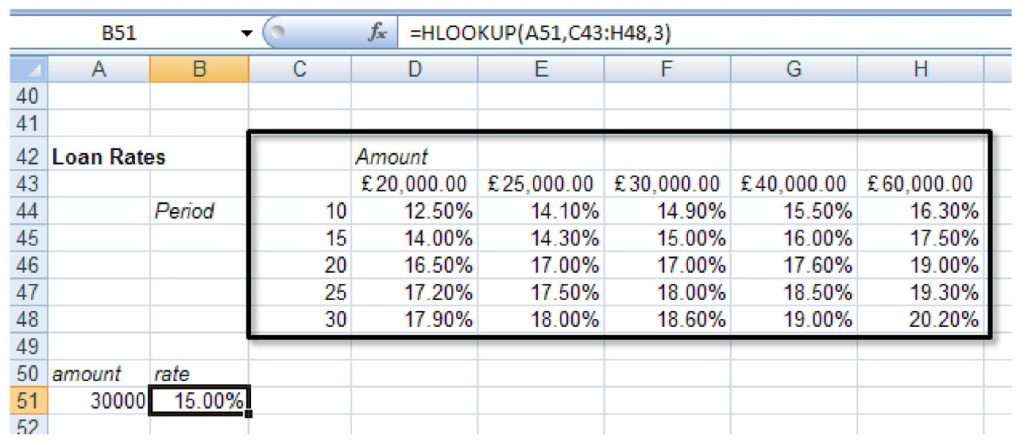
Whatever the amount a customer wants to borrow, he may pay up to five different rates of interest depending on whether the loan is over 10, 15 or more years. The HLOOKUP function will find a specific amount, then move down the array to find the appropriate interest rate for the required time period.

Designate cell A51 as the cell to hold the amount, i.e. the LOOKUP_VALUE; cells C43:H48 are the TABLE_ARRAY; the ROW_INDEX_NUMBER will be 2 if a customer wants the loan over 10 years, 3 if he wants the loan over 15 years, and so on. Cell B51 holds this formula;

=HLOOKUP(A51,C43:H48,3)

The above formula looks along the top row of the array for the value in cell A51 (30000). It then moves down to row 3 and returns the value 15.00%, which is the correct interest rate for a £30000 loan over 15 years. (Range names could be used here to simplify the formula).

As with the LOOKUP function, the advantage of HLOOKUP is that it does not necessarily have to find the exact LOOKUP_VALUE. If, for example, you wanted to find out what interest rate is applicable to a £28000 loan, the figure 28000 can be entered in the LOOKUP_VALUE cell (A51) and the rate 14.30% appears. As before, Excel has looked for the value in the array closest to, but lower than, the LOOKUP_VALUE.

Vlookup

The VLOOKUP function works on the same principle as HLOOKUP, but instead of searching horizontally, VLOOKUP searches vertically. VLOOKUP searches for a specified value vertically down the first column of an array. When the value is found, VLOOKUP searches across to a specified column and enters the value of the cell. The syntax for the VLOOKUP function follows the same pattern as HLOOKUP, except that instead of specifying a row index number, you would specify a column index number to instruct VLOOKUP to move across to a specific column in the array where the required value is to be found.

=VLOOKUP( lookup_value , table_array , col_index_number )

In the case of VLOOKUP, data in the first column of the array should be in ascending order, as VLOOKUP searches down this column for the LOOKUP_VALUE.

In the same spreadsheet, a VLOOKUP formula could be used to search for a specific time period, then return the appropriate rate for a fixed amount. In the following example, a time period is entered in cell A54 and in B54 the VLOOKUP formula is contained;

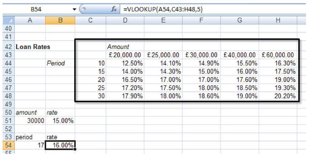
Cell B54 holds this formula;

=VLOOKUP(A54,C43:H48,5)

The cell A54 is the LOOKUP_VALUE (time period), the TABLE_ARRAY is as before, and for this example rates are looked up for a loan of £40000, hence the COLUMN_INDEX_NUMBER5. By changing the value of cell A54, the appropriate rate for that time period is returned. Where the specific lookup_value is not found, VLOOKUP works in the same way as HLOOKUP. In other words, the nearest value in the array that is less than the LOOKUP_VALUE will be returned. So, a £40000 loan over 17 years would return an interest rate of 16.00%.